Electrons in a Weak Periodic Potential
Electrons in a Weak Periodic Potential: Band Gaps and Bragg Planes
The free-electron model treats conduction electrons as particles moving through a metal with negligible influence from the ions. This model explains several metallic properties, but it cannot account for one of the central features of crystalline solids: the electronic spectrum forms energy bands, and these bands may be separated by energy gaps.
A systematic improvement is obtained by starting from the Sommerfeld free-electron model and adding a weak periodic potential produced by the crystal lattice. This approach is called the nearly-free-electron model. Its central result is that the periodic potential produces only small corrections to most free-electron states, but it has a strong effect near Bragg planes, where free-electron states become degenerate or nearly degenerate. At these planes, free-electron parabolas that would cross in the absence of a lattice potential repel each other, producing band gaps.
The purpose of this post is to derive this result from the Schrödinger equation, interpret the origin of the energy gap, and connect the one-dimensional picture to Brillouin zones, Fermi surfaces, and structure factors.
Why the crystal potential can be treated as weak
At first sight, treating the crystal potential as weak may appear surprising. The ions in a crystal are positively charged, so the bare electron-ion interaction can be strong. However, the nearly-free-electron approximation is based on the effective potential felt by conduction electrons, not on the unscreened ionic potential. Two main reasons make this approximation reasonable.
First, conduction electrons are not allowed to spend much time right on top of the ions. The core-electron states near the ions are already occupied, and the Pauli principle prevents the conduction electrons from simply collapsing into those regions.
Second, conduction electrons are mobile. They rearrange around positive ions and partially cancel the ion fields. This is screening. So the electron does not feel the bare ionic potential; it feels an effective potential that is much smoother and weaker.
The model is therefore
$ \text{Sommerfeld free electron gas} \quad + \quad \text{weak periodic lattice potential}. $
The potential is weak, but it is not random. Its periodicity is the essential feature responsible for the formation of band gaps.
Start with the Schrödinger equation
The one-electron Schrödinger equation is
$ \left[-\frac{\hbar^2}{2m}\nabla^2+U(\mathbf r)\right]\psi(\mathbf r) =\varepsilon\psi(\mathbf r), $
where
$ U(\mathbf r+\mathbf R)=U(\mathbf r) $
for every Bravias lattice vector $\mathbf R$.
Because the potential is periodic, it is natural to expand it in reciprocal-lattice vectors:
$ U(\mathbf r)=\sum_{\mathbf K}U_{\mathbf K}e^{i\mathbf K\cdot\mathbf r}. $
The Fourier coefficient is
$ U_{\mathbf K} =\frac{1}{v}\int_{\text{cell}}d\mathbf r\, e^{-i\mathbf K\cdot\mathbf r}U(\mathbf r), $
where $v$ is the primitive-cell volume.
If $U(\mathbf r)$ is real, then
$ U_{-\mathbf K}=U^*_{\mathbf K}. $
If the crystal also has inversion symmetry, $U(\mathbf r)=U(-\mathbf r)$, then the relevant Fourier coefficients can be chosen real.
In the free-electron problem, the eigenstates are plane waves. Since the periodic potential is weak, one writes the exact Bloch wave as a superposition of plane waves whose wavevectors differ by reciprocal-lattice vectors:
$ \psi_{\mathbf q}(\mathbf r) =\sum_{\mathbf K}C_{\mathbf q-\mathbf K} e^{i(\mathbf q-\mathbf K)\cdot\mathbf r}. $
Here $\mathbf q$ is the crystal momentum label, and $\mathbf K$ runs over reciprocal-lattice vectors.
For each plane-wave component, the free-electron energy is
$ \varepsilon^0_{\mathbf q-\mathbf K} =\frac{\hbar^2|\mathbf q-\mathbf K|^2}{2m}. $
Substituting the plane-wave expansion into the Schrödinger equation gives the central equation:
$ \left[\varepsilon^0_{\mathbf q-\mathbf K}-\varepsilon\right] C_{\mathbf q-\mathbf K} + \sum_{\mathbf K'}U_{\mathbf K'-\mathbf K} C_{\mathbf q-\mathbf K'}=0. $
Equivalently,
$ \left[\varepsilon-\varepsilon^0_{\mathbf q-\mathbf K}\right] C_{\mathbf q-\mathbf K} = \sum_{\mathbf K'}U_{\mathbf K-\mathbf K'} C_{\mathbf q-\mathbf K'}. $
This equation shows that the lattice potential mixes plane waves whose wavevectors differ by reciprocal-lattice vectors. This is the wave-mechanical form of Bragg scattering. If $U=0$, the central equation becomes
$ \left[\varepsilon-\varepsilon^0_{\mathbf q-\mathbf K}\right] C_{\mathbf q-\mathbf K}=0. $
A coefficient can therefore be nonzero only if
$ \varepsilon=\varepsilon^0_{\mathbf q-\mathbf K}. $
If there is no degeneracy, only one coefficient survives, and the wavefunction is just one plane wave:
$ \psi(\mathbf r)=e^{i(\mathbf q-\mathbf K_1)\cdot\mathbf r}. $
If two or more free-electron energies are equal or nearly equal, the weak periodic potential can mix them strongly. This is the regime in which the weak perturbation has its largest qualitative effect.
Nondegenerate case: second-order energy shifts
Fix $\mathbf q$ and focus on one reciprocal-lattice vector $\mathbf K_1$. Suppose its free-electron energy is far from all the others on the scale of the weak potential:
$ \left| \varepsilon^0_{\mathbf q-\mathbf K_1} - \varepsilon^0_{\mathbf q-\mathbf K} \right|\gg U, \qquad \mathbf K\ne\mathbf K_1. $
Then the weak lattice potential cannot strongly mix this state with the others. The other coefficients are small. To leading order,
$ C_{\mathbf q-\mathbf K} \approx \frac{U_{\mathbf K_1-\mathbf K}C_{\mathbf q-\mathbf K_1}} {\varepsilon-\varepsilon^0_{\mathbf q-\mathbf K}}, \qquad \mathbf K\ne\mathbf K_1. $
Putting this back into the equation for the main coefficient gives the energy shift
$ \varepsilon = \varepsilon^0_{\mathbf q-\mathbf K_1} + \sum_{\mathbf K\ne\mathbf K_1} \frac{|U_{\mathbf K-\mathbf K_1}|^2} {\varepsilon^0_{\mathbf q-\mathbf K_1}-\varepsilon^0_{\mathbf q-\mathbf K}} +O(U^3). $
The important consequence is the order of the correction:
$ \Delta\varepsilon \sim U^2. $
Thus, away from degeneracies, a weak periodic potential produces only a second-order correction. The energy bands remain almost free-electron-like.
Nearly degenerate case: first-order splitting
Now suppose several free-electron levels are close together:
$ \varepsilon^0_{\mathbf q-\mathbf K_1},\quad \varepsilon^0_{\mathbf q-\mathbf K_2},\quad \ldots,\quad \varepsilon^0_{\mathbf q-\mathbf K_m}. $
They are close to one another on the scale of $U$, but far from all other free-electron levels:
$ \left| \varepsilon^0_{\mathbf q-\mathbf K_i} - \varepsilon^0_{\mathbf q-\mathbf K} \right|\gg U, \qquad \mathbf K\notin\{\mathbf K_1,\ldots,\mathbf K_m\}. $
Then the coefficients inside this nearly degenerate set must be solved together:
$ \left(\varepsilon-\varepsilon^0_{\mathbf q-\mathbf K_i}\right) C_{\mathbf q-\mathbf K_i} = \sum_{j=1}^{m} U_{\mathbf K_i-\mathbf K_j}C_{\mathbf q-\mathbf K_j}. $
This is degenerate perturbation theory in the plane-wave basis. In this case the energy splitting is first order:
$ \Delta\varepsilon \sim U. $
Therefore, weak periodic potentials are most important near degeneracies.
Two level mixing
The simplest important case occurs when only two free-electron plane waves are nearly degenerate:
$ \mathbf q \quad\text{and}\quad \mathbf q-\mathbf K. $
The coupled equations are
$ (\varepsilon-\varepsilon^0_{\mathbf q})C_{\mathbf q} =U^*_{\mathbf K}C_{\mathbf q-\mathbf K}, $
$ (\varepsilon-\varepsilon^0_{\mathbf q-\mathbf K})C_{\mathbf q-\mathbf K} =U_{\mathbf K}C_{\mathbf q}. $
For a nonzero solution, the determinant must vanish:
$ \begin{vmatrix} \varepsilon-\varepsilon^0_{\mathbf q} & -U^*_{\mathbf K}\\ -U_{\mathbf K} & \varepsilon-\varepsilon^0_{\mathbf q-\mathbf K} \end{vmatrix}=0. $
Therefore
$ (\varepsilon-\varepsilon^0_{\mathbf q}) (\varepsilon-\varepsilon^0_{\mathbf q-\mathbf K}) =|U_{\mathbf K}|^2. $
Solving the quadratic gives
$ \varepsilon_{\pm} = \frac{1}{2} \left(\varepsilon^0_{\mathbf q}+\varepsilon^0_{\mathbf q-\mathbf K}\right) \pm \left[ \left( \frac{\varepsilon^0_{\mathbf q}-\varepsilon^0_{\mathbf q-\mathbf K}}{2} \right)^2 +|U_{\mathbf K}|^2 \right]^{1/2}. $
This expression describes an avoided crossing. Without the periodic potential, the two free-electron branches cross. With the periodic potential, the branches repel.
What is a Bragg Plane
The two free-electron levels are degenerate when
$ \varepsilon^0_{\mathbf q}=\varepsilon^0_{\mathbf q-\mathbf K}. $
Since
$ \varepsilon^0_{\mathbf q}=\frac{\hbar^2q^2}{2m}, $
the degeneracy condition is
$ q^2=|\mathbf q-\mathbf K|^2. $
Expand the right-hand side:
$ q^2=q^2-2\mathbf q\cdot\mathbf K+K^2. $
So
$ \mathbf q\cdot\mathbf K=\frac{K^2}{2}, $
or
$ \left(\mathbf q-\frac{\mathbf K}{2}\right)\cdot\mathbf K=0. $
This means $\mathbf q-\mathbf K/2$ is perpendicular to $\mathbf K$. Geometrically, the degeneracy occurs on the plane perpendicular to $\mathbf K$ and halfway between $0$ and $\mathbf K$.
That plane is the Bragg plane.
This terminology is connected to diffraction. The same geometric condition appears in Bragg reflection: the periodic lattice couples waves whose momenta differ by a reciprocal-lattice vector.
On the Bragg plane,
$ \varepsilon^0_{\mathbf q}=\varepsilon^0_{\mathbf q-\mathbf K}\equiv\varepsilon^0. $
Then the two-level energies reduce to
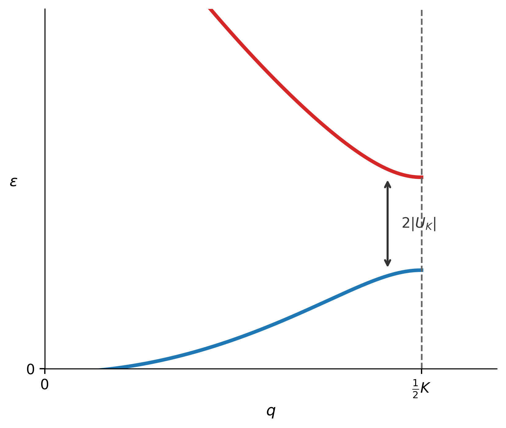
$ \varepsilon_{\pm}=\varepsilon^0\pm |U_{\mathbf K}|. $
Therefore the energy gap is
$ \Delta\varepsilon =\varepsilon_+-\varepsilon_- =2|U_{\mathbf K}|. $
This is the central result of the weak-periodic-potential model:
The Fourier component $U_{\mathbf K}$ opens a gap of size $2|U_{\mathbf K}|$ at the Bragg plane associated with $\mathbf K$.
Therefore, not every Fourier component of the potential affects every gap. The gap at a given Bragg plane is controlled specifically by the Fourier component associated with that reciprocal-lattice vector.
If
$ U_{\mathbf K}=0, $
then there is no first-order gap at that Bragg plane.
At the Bragg plane, the two waves $e^{i\mathbf q\cdot\mathbf r}$ and $e^{i(\mathbf q-\mathbf K)\cdot\mathbf r}$ have the same free-electron energy. The lattice mixes them into symmetric and antisymmetric combinations.
Assume $U_{\mathbf K}$ is real and positive. For the upper level,
$ \varepsilon=\varepsilon^0+|U_{\mathbf K}|, $
and the coefficients have the same sign:
$ C_{\mathbf q}=C_{\mathbf q-\mathbf K}. $
So the wavefunction is approximately
$ \psi_+(\mathbf r)\propto e^{i\mathbf q\cdot\mathbf r} +e^{i(\mathbf q-\mathbf K)\cdot\mathbf r}. $
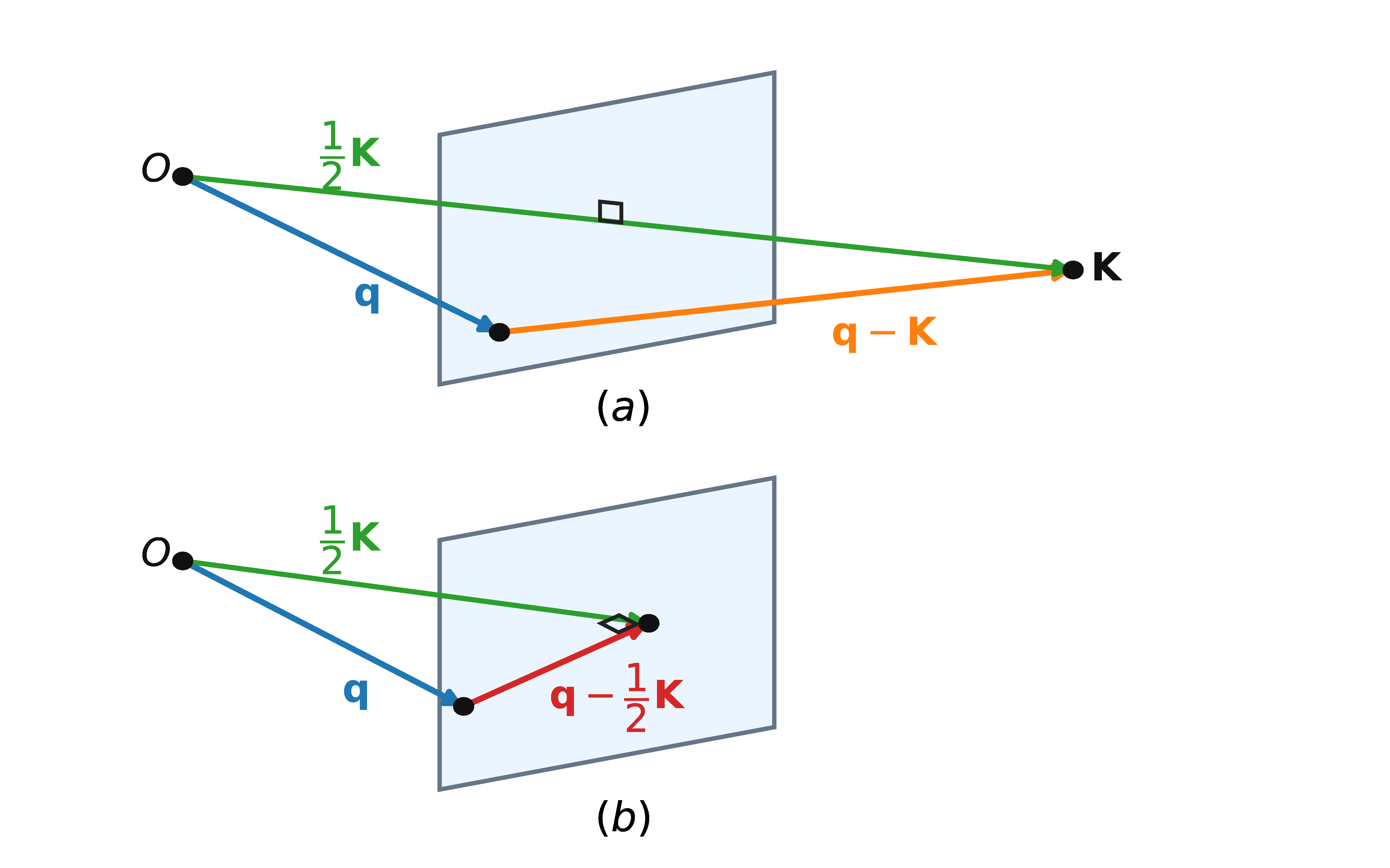
On the Bragg plane write
$ \mathbf q=\frac{\mathbf K}{2}+\mathbf p, \qquad \mathbf p\cdot\mathbf K=0. $
Then
$ \mathbf q-\mathbf K=-\frac{\mathbf K}{2}+\mathbf p. $
Ignoring the common phase $e^{i\mathbf p\cdot\mathbf r}$, the upper state is a standing wave with density
$ |\psi_+(\mathbf r)|^2\propto \cos^2\left(\frac{\mathbf K\cdot\mathbf r}{2}\right). $
The lower state has the opposite relative sign and density
$ |\psi_-(\mathbf r)|^2\propto \sin^2\left(\frac{\mathbf K\cdot\mathbf r}{2}\right). $
This explains the usual s-like / p-like description of the states at the gap. One standing wave has charge density concentrated where the other has nodes. Since the two states place electron density differently relative to the ion planes, they have different potential energies. That difference is the gap.
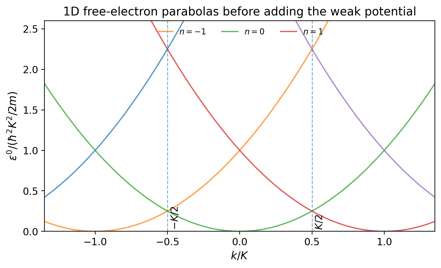
In one dimension, the free-electron energy is
$ \varepsilon^0_k=\frac{\hbar^2k^2}{2m}. $
The reciprocal-lattice vectors are
$ K=\frac{2\pi n}{a}. $
The Bragg points are halfway to reciprocal-lattice points:
$ k=\frac{K}{2}=\frac{\pi n}{a}. $
At these points, the original free-electron parabola intersects a shifted parabola,
$ \frac{\hbar^2}{2m}|k-K|^2. $
Without the lattice potential, the parabolas cross.
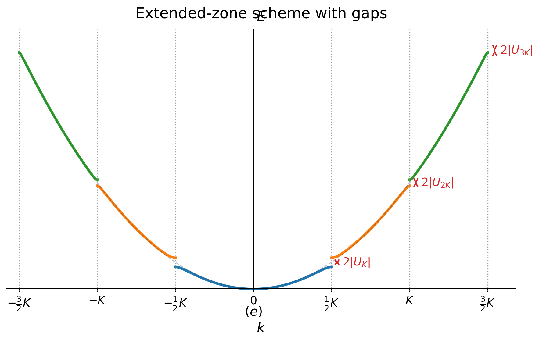
With the weak periodic potential, the crossing becomes an avoided crossing. The gap size is
$ 2|U_K|. $
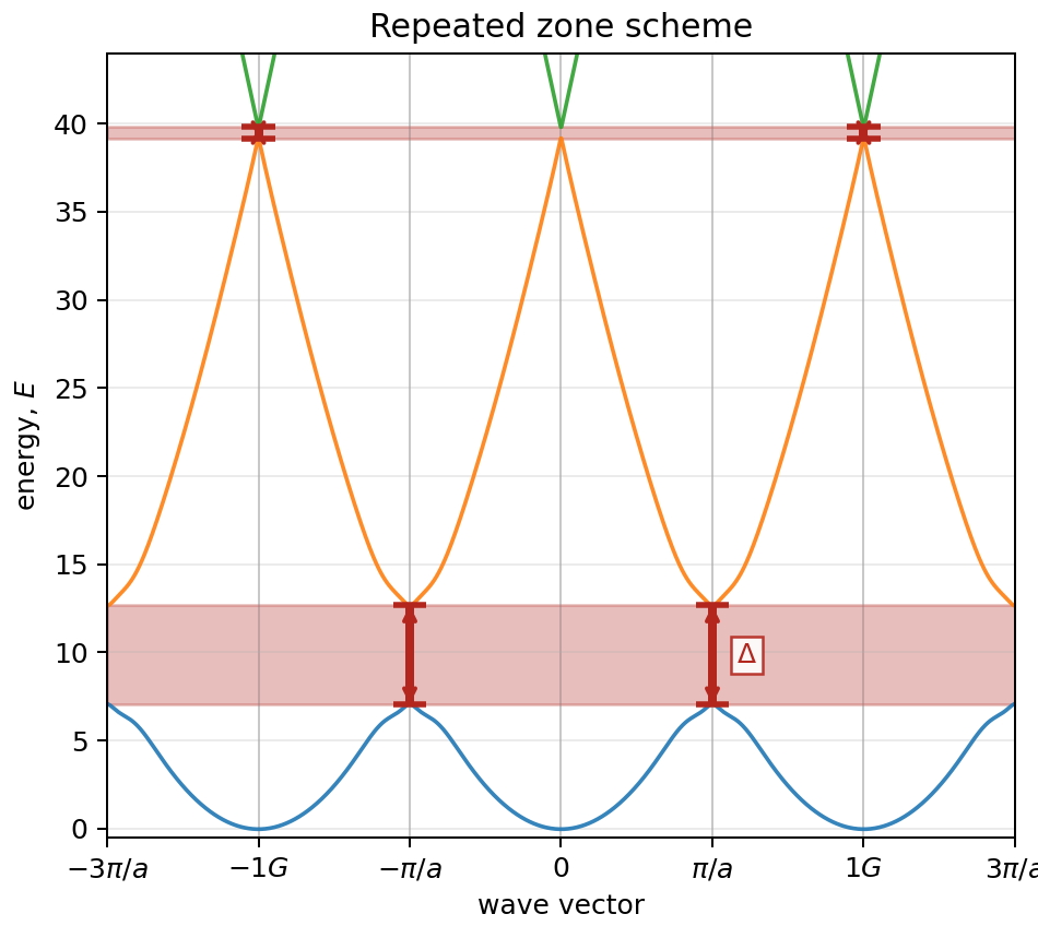
This gives the basic picture of band formation: the free-electron parabola is copied by reciprocal-lattice translations, and small gaps open where the copies intersect.
The same band structure can be drawn in different ways. The physics is the same; only the labeling changes.
In the extended-zone scheme, the bands are followed continuously in $k$-space. This makes the avoided crossings easy to see.
In the reduced-zone scheme, every state is folded back into the first Brillouin zone. Instead of one long curve through many zones, one obtains several bands inside one zone.
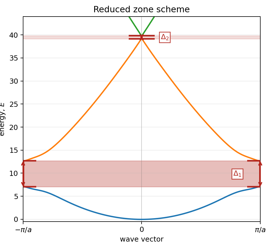
There is also the repeated-zone scheme, where the reduced-zone picture is periodically repeated throughout reciprocal space. It is redundant, because the same level appears at equivalent wavevectors, but it is useful for visualizing symmetry.
Energy curves in three dimensions
In three dimensions, the full band structure is a function
$ \varepsilon_n(\mathbf k), $
which is difficult to draw completely. Therefore, it is customary to plot energy along selected lines in reciprocal space, often along high-symmetry directions.
A useful caution is that those plotted paths are not necessarily periodic by themselves. They are just useful cuts through the Brillouin zone. A band diagram is therefore not the whole function $\varepsilon_n(\mathbf k)$; it is a carefully chosen slice through it.
Fermi surfaces and Brillouin zones
For metals, the most important states are usually near the Fermi surface. In the weak-potential picture, the construction is:
- Draw the free-electron Fermi sphere centered at $\mathbf k=0$.
- Find where it crosses Bragg planes.
- At those crossings, open gaps and deform the Fermi surface.
This turns the free-electron sphere into a fractured and rounded surface in reciprocal space.
Brillouin zones organize this geometry. The first Brillouin zone is the region that can be reached from the origin without crossing a Bragg plane. The second zone is reached by crossing one Bragg plane. More generally:
$ \text{the } n\text{th Brillouin zone is reached by crossing } n-1 \text{ Bragg planes, but no fewer.} $
This explains why Brillouin-zone boundaries are physically special. Inside a zone, the weak potential changes free-electron energies only in second order. At a zone boundary, which is a Bragg plane, it changes them in first order.
Each Brillouin zone is also a primitive cell of the reciprocal lattice.
Why structure factors control gaps
The final point is the origin of the Fourier coefficient $U_{\mathbf K}$. Its size is determined by both the atomic potential and the geometry of the basis.
Suppose the periodic potential is made by adding identical atomic potentials centered at ion positions. If the basis atoms inside one primitive cell are at positions $\mathbf d_j$, then
$ U(\mathbf r)=\sum_{\mathbf R}\sum_j \phi(\mathbf r-\mathbf R-\mathbf d_j), $
where $\phi$ is the potential of one ion.
The Fourier coefficient is
$ U_{\mathbf K} =\frac{1}{v}\int_{\text{cell}}d\mathbf r\, e^{-i\mathbf K\cdot\mathbf r}U(\mathbf r). $
Substitution gives
$ U_{\mathbf K} =\frac{1}{v}\phi(\mathbf K)S_{\mathbf K}, $
where
$ \phi(\mathbf K)=\int_{\text{all space}}d\mathbf r\, e^{-i\mathbf K\cdot\mathbf r}\phi(\mathbf r) $
is the Fourier transform of the atomic potential, and
$ S_{\mathbf K}=\sum_j e^{-i\mathbf K\cdot\mathbf d_j} $
is the geometrical structure factor. The sign in the exponential depends on the Fourier convention, but the physical condition $S_{\mathbf K}=0$ does not.
This gives an important result:
$ S_{\mathbf K}=0 \quad\Longrightarrow\quad U_{\mathbf K}=0 \quad\Longrightarrow\quad \text{no first-order gap at that Bragg plane.} $
Thus, the same basis geometry that creates missing peaks in diffraction can also remove first-order band gaps in the nearly-free-electron model.
Key results
- The weak periodic potential is plausible because conduction electrons avoid core regions and screen ion fields.
- A periodic potential couples plane waves whose wavevectors differ by reciprocal-lattice vectors.
- Away from degeneracies, energy shifts are second order in $U$.
- Near Bragg planes, free-electron states become degenerate or nearly degenerate.
- At a single Bragg plane, the band gap is
$ \Delta=2|U_{\mathbf K}|. $
- The Bragg plane for $\mathbf K$ satisfies
$ \left(\mathbf q-\frac{\mathbf K}{2}\right)\cdot\mathbf K=0. $
- In 1D, gaps open at
$ k=\frac{K}{2}=\frac{\pi n}{a}. $
- The structure factor controls which Fourier components of the lattice potential vanish, so it also controls which first-order gaps vanish.